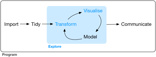
Data Manipulation

Data manipulation, pre-processing and cleaning might not be the most glamourous component of data analysis, but is nonetheless essential to any statistical (or machine learning!) analysis. Being able to efficiently and neatly process data is thus an important topic, for which we try here to provide a few basic elements — focusing on its implementation with R.

We will focus here on:

The “purrr” package , for efficient data manipulations (loops over the data, etc),
Handling missing values
Merging datasets
Exporting data

1. The "purrr" package

The package purrr is part of the tidyverse suit (and is consequently automatically downloaded by calling the tidyverse). purrr handles tasks similar to ones performed by apply-family functions in base R through a family of “map” functions (see details below).

It enhances R’s functional programming toolkit by providing a complete and consistent set of tools for working with functions and vectors.

1.1 The map functions

map-functions allow you to replace many for loops with code that is easier to read. purrr functions are implemented in C, which can also make it more efficient that manual loops over the data.
For instance:

map(), map_if(), map_at() returns a list
map_lgl() returns a logical vector,
map_int() returns a integer vector,
map_dbl() returns a double vector,
map_chr() returns a character vector,
map_dfr(), map_dfc() returns a data.frame by binding rows or columns respectively.

Example: column-wise mean

df <- tibble(a=rnorm(10), b=rnorm(10), c=rnorm(10), d=rnorm(10))
map_dbl(df, mean)                       # or equivalently: df %>% map_dbl(mean)

The focus here is on the operation being performed, not the book-keeping. The second argument, .f, can be a functions, a formula, a character vector, or an integer vector.

map(1:3, ~ rnorm(7, .x))

map can pass additional parameters to the function:

map_dbl(df, mean, trim = 0.25)

mtcars %>% 
  split(.$cyl)

mtcars %>% 
  split(.$cyl) %>%
  map_df(dim)

1.2. Base-R maps vs. purrr maps

purrr does some of the same than the apply family. However, purrr is more consistent, so you should learn it.

A quick reference of similar base R functions:

lapply is basically identical to map.
sapply is a wrapper around lapply and it tries to simplify the output. Downside: you never know what you’ll get.
vapply: like sapply, but you can supply an additional argument that defines the type.

You can learn more about purrr here: (http://r4ds.had.co.nz/iteration.html).

2. Handling missing values

2.1. Types of Missingness

There are two main types of missingness: explicit and implicit, as showcased in the following example.

stocks <- tibble(
  year   = c(2015, 2015, 2015, 2015, 2016, 2016, 2016),
  qtr    = c(   1,    2,    3,    4,    2,    3,    4),
  return = c(1.88, 0.59, 0.35,   NA, 0.92, 0.17, 2.66)
)

The return for the fourth quarter of 2015 is explicitly missing.
The return for the first quarter of 2016 is implicitly missing.

The way that a dataset is represented can make implicit values explicit.

stocks %>% spread(year, return)

2.2 Gathering missing data

Recall the functions we learned from tidyr package.

You can used spread() and gather() to retain only non-missing recored, i.e. to turn all explicit missing values into implicit ones.

stocks %>% spread(year, return) %>% 
  gather(year, return, `2015`:`2016`, na.rm = TRUE)

2.3 Completing missing data

complete() takes a set of columns, and finds all unique combinations. It then ensures the original dataset contains all those values, filling in explicit NAs where necessary.

stocks %>% complete(year, qtr)

2.4 Different intepretations of `NA`

Sometimes when a data source has primarily been used for data entry, missing values indicate that the previous value should be carried forward:

# tribble() constructs a tibble by filling by rows
treatment <- tribble(
  ~ person,           ~ treatment, ~response,
  "Derrick Whitmore", 1,           7,
  NA,                 2,           10,
  NA,                 3,           9,
  "Katherine Burke",  1,           4
)

You can fill in these missing values with fill()

treatment %>% fill(person)

3. Merging datasets

3.1 Relational data

Rarely does a data analysis involve only a single table of data.
Collectively, multiple tables of data are called relational data because the relations, not just the individual datasets, that are important.
Relations are always defined between a pair of tables.
All other relations are built up from this simple idea: the relations of three or more tables are always a property of the relations between each pair.

Example: The nycflights13 package contains a collection of related datasets.

library(nycflights13)

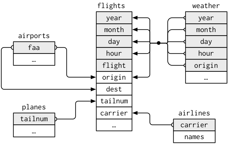
Source: (http://r4ds.had.co.nz/relational-data.html)

3.2. Keys

A key is a variable (or set of variables) that uniquely identifies an observation.

For example, each plane is uniquely determined by its tailnum, but an observation in ‘weather’ is identified by five variables: year, month, day, hour, and origin

Keys can be used to connect each pair of tables together.

There are two types of keys:

Primary: identifies an observation in its own table. Example: planes$tailnum
Foreign: identifies an observation in another table. Example: flights$tailnum, this is because tailnum does not enough to identify a record in flights dataset.

A variable can be both a primary key and a foreign key.

Identify primary keys

It’s good practice to verify that chosen keys do indeed uniquely identify each observation.

One way to do that is to count() the primary keys and look for entries where n is greater than one:

planes %>% 
  count(tailnum) %>% 
  filter(n > 1)

weather %>% 
  count(year, month, day, hour, origin) %>% 
  filter(n > 1)

No primary key

Sometimes a table doesn’t have an explicit primary key, e.g. in flights dataset each row is an observation, but no combination of variables reliably identifies it, (even the flight numbers).

In this case, you can add an extra identifier column:

flights %>% 
  count(flight) %>% 
  filter(n > 1)

flights %>%
  mutate(flight_id= paste0("F", row_number())) %>%
  select(flight_id, year:flight)

3.3. Merging two tables

There are three families of functions designed to merge relational data:

Mutating joins, which add new variables to one data frame from matching observations in another.
Filtering joins, which filter observations from one data frame based on whether or not they match an observation in the other table.
Set operations, which treat observations as if they were set elements.

3.3.a. Mutating joins

A mutating join allows you to combine variables from two tables, by matching observations by their keys, and then copying across variables from one table to the other. e.g.

flights %>%
  select(year:day, hour, origin, dest, tailnum, carrier) %>% 
  left_join(airlines, by = "carrier")

There are four mutating join functions:

inner_join()
outer joins;
- left_join()
- right_join()
- full_join()

A simple example:

x <- tribble(
  ~key, ~val_x,
     1, "x1",
     2, "x2",
     3, "x3"
)


y <- tribble(
  ~key, ~val_y,
     1, "y1",
     2, "y2",
     4, "y3"
)

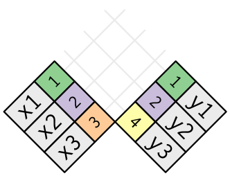
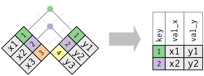
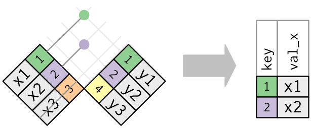
Inner join

x %>% inner_join(y, by = "key")

Source: (http://r4ds.had.co.nz/relational-data.html)

Outer join

An outer join keeps observations that appear in at least one of the tables:

A 'left_join()' keeps all observations in the table on the left

A 'right_join()' keeps all observations in the table on the right

A 'full_join()' keeps all observations in both tables

Source: http://r4ds.had.co.nz/relational-data.html

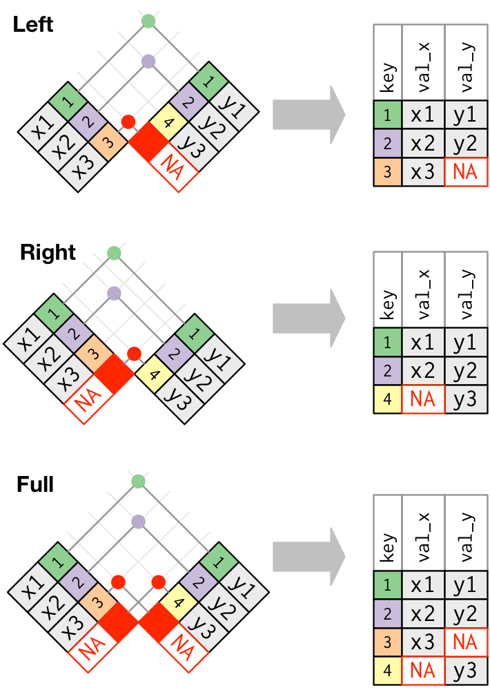
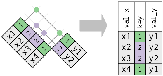
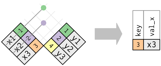
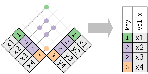
Duplicate keys

What happens when there are duplicate keys?

One table has duplicate keys. There may be a one-to-many relation.

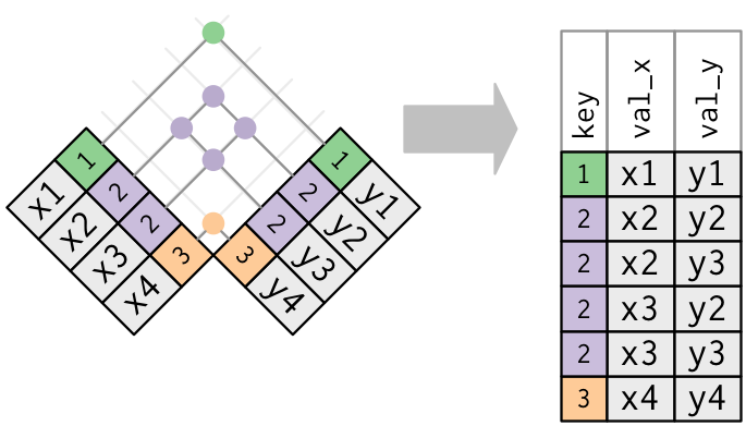
Both tables have duplicate keys. When you join duplicated keys, you get all possible combinations:

Source: http://r4ds.had.co.nz/relational-data.html

3.3.b. Filtering joins

Filtering joins match observations in the same way as mutating joins, but affect the observations, not the variables.

There are two types:

semi_join(x, y) keeps all observations in x that have a match in y.
anti_join(x, y) drops all observations in x that have a match in y.

Multiple matches

In filtering joins, only the existence of a match is important.

It doesn’t matter which observation is matched.

Filtering joins never duplicate rows like mutating joins do:

3.3.c. Set operations

Set operations apply to rows; they expect the x and y inputs to have the same variables, and treat the observations like sets.

intersect(x, y): returns only observations in both x and y.
union(x, y): returns unique observations in x and y.
setdiff(x, y): returns observations in x, but not in y.

All these operations work with a complete row, comparing the values of every variable.
Examples:

df1 <- tribble(
  ~x, ~y,
   1,  1,
   2,  1
)
df2 <- tribble(
  ~x, ~y,
   1,  1,
   1,  2
)

intersect(df1, df2)

union(df1, df2)
setdiff(df1, df2)
setdiff(df2, df1)

4. Data Export

4.1 Exporting Data

After working with a dataset and doing all data manipulation, you might want to save your new data table.

Recall the readr package. Besides functions for reading data in, readr has utilities for saving your data to a text file:

write_tsv(mydata, "path/to/filename.tsv")                  # tab-delimited
write_csv(mydata, "path/to/filename.csv")                  # comma-delimited
write_delim(mydata, "path/to/filename.csv", delim = " ")   # general delimiter

To save your data in other types of files, you need to install and use other packages:

to export an Excel spreadsheet, use xlsx package, and follow this guide.

# install.packages(xlsx)
library(xlsx)
write.xlsx(mydata, "path/to/filename.xlsx")

to export SAS, SPSS and Stata files use the haven package.

# install.packages(haven)
library(haven)
read_sas("mtcars.sas7bdat")
write_sas(mtcars, "mtcars.sas7bdat")

4.2. Saving the workspace

You can also choose to save all objects currently in the workspace (variables, functions, etc.) into a file e.g. filename.rda.
The file filename.rda can be the easily loaded next time you work with R.
You can also save a single object or a subset of specified objects currently in the workspace.

# save the workspace to file 
save.image(file = "path/to/filename.rda")

# save specific objects to a file
save(object_list, file = "path/to/filename.rda")

# save just a single object
saveRDS(object, file = "path/to/filename.rds")

Saved objects/workspace can be loaded back in a new R session.

# load a workspace into the current session
load("path/to/filename.rda")

# read just the previously saved 1 object
object <- readRDS("path/to/filename.rds")

Based on the R-bootcamp class by Lan Huong Nguyen (Stanford), edited by Claire Donnat.

Statistical Consulting Program